PyPy is a Python implementation and a dynamic language implementation framework.
This chapter assumes familiarity with some basic interpreter and compiler concepts like bytecode and constant folding.
Python is a high-level, dynamic programming language. It was invented by the Dutch programmer Guido van Rossum in the late 1980s. Guido's original implementation is a traditional bytecode interpreter written in C, and consequently known as CPython. There are now many other Python implementations. Among the most notable are Jython, which is written in Java and allows for interfacing with Java code, IronPython, which is written in C# and interfaces with Microsoft's .NET framework, and PyPy, the subject of this chapter. CPython is still the most widely used implementation and currently the only one to support Python 3, the next generation of the Python language. This chapter will explain the design decisions in PyPy that make it different from other Python implementations and indeed from any other dynamic language implementation.
PyPy, except for a negligible number of C stubs, is written completely in Python. The PyPy source tree contains two major components: the Python interpreter and the RPython translation toolchain. The Python interpreter is the programmer-facing runtime that people using PyPy as a Python implementation invoke. It is actually written in a subset of Python called Restricted Python (usually abbreviated RPython). The purpose of writing the Python interpreter in RPython is so the interpreter can be fed to the second major part of PyPy, the RPython translation toolchain. The RPython translator takes RPython code and converts it to a chosen lower-level language, most commonly C. This allows PyPy to be a self-hosting implementation, meaning it is written in the language it implements. As we shall see throughout this chapter, the RPython translator also makes PyPy a general dynamic language implementation framework.
PyPy's powerful abstractions make it the most flexible Python implementation. It has nearly 200 configuration options, which vary from selecting different garbage collector implementations to altering parameters of various translation optimizations.
Since RPython is a strict subset of Python, the PyPy Python interpreter can be run on top of another Python implementation untranslated. This is, of course, extremely slow but it makes it possible to quickly test changes in the interpreter. It also enables normal Python debugging tools to be used to debug the interpreter. Most of PyPy's interpreter tests can be run both on the untranslated interpreter and the translated interpreter. This allows quick testing during development as well as assurance that the translated interpreter behaves the same as the untranslated one.
For the most part, the details of the PyPy Python interpreter are quite similiar
to that of CPython; PyPy and CPython use nearly identical bytecode and data
structures during interpretation. The primary difference between the two is PyPy
has a clever abstraction called object spaces (or objspaces for
short). An objspace encapsulates all the knowledge needed to represent and
manipulate Python data types. For example, performing a binary operation on two
Python objects or fetching an attribute of an object is handled completely by
the objspace. This frees the interpreter from having to know anything about the
implementation details of Python objects. The bytecode interpreter treats Python
objects as black boxes and calls objspace methods whenever it needs to
manipulate them. For example, here is a rough implementation of the
BINARY_ADD opcode, which is called when two objects are combined with the
+ operator. Notice how the operands are not inspected by the interpreter; all
handling is delegated immediately to the objspace.
def BINARY_ADD(space, frame):
    object1 = frame.pop() # pop left operand off stack
    object2 = frame.pop() # pop right operand off stack
    result = space.add(object1, object2) # perform operation
    frame.push(result) # record result on stack
The objspace abstraction has numerous advantages. It allows new data type implementations to be swapped in and out without modifying the interpreter. Also, since the sole way to manipulate objects is through the objspace, the objspace can intercept, proxy, or record operations on objects. Using the powerful abstraction of objspaces, PyPy has experimented with thunking, where results can be lazily but completely transparently computed on demand, and tainting, where any operation on an object will raise an exception (useful for passing sensitive data through untrusted code). The most important application of objspaces, however, will be discussed in Section 19.4.
The objspace used in a vanilla PyPy interpreter is called the standard objspace (std objspace for short). In addition to the abstraction provided by the objspace system, the standard objspace provides another level of indirection; a single data type may have multiple implementations. Operations on data types are then dispatched using multimethods. This allows picking the most efficient representation for a given piece of data. For example, the Python long type (ostensibly a bigint data type) can be represented as a standard machine-word-sized integer when it is small enough. The memory and computationally more expensive arbitrary-precision long implementation need only be used when necessary. There's even an implementation of Python integers available using tagged pointers. Container types can also be specialized to certain data types. For example, PyPy has a dictionary (Python's hash table data type) implementation specialized for string keys. The fact that the same data type can be represented by different implementations is completely transparent to application-level code; a dictionary specialized to strings is identical to a generic dictionary and will degenerate gracefully if non-string keys are put into it.
PyPy distinguishes between interpreter-level (interp-level) and
application-level (app-level) code. Interp-level code, which most of the
interpreter is written in, must be in RPython and is translated. It directly
works with the objspace and wrapped Python objects. App-level code is always run
by the PyPy bytecode interpreter. As simple as interp-level RPython code is,
compared to C or Java, PyPy developers have found it easiest to use pure app-level
code for some parts of the interpreter. Consequently, PyPy has support for
embedding app-level code in the interpreter. For example, the functionality of
the Python print statement, which writes objects to standard output, is
implemented in app-level Python. Builtin modules can also be written partially
in interp-level code and partially in app-level code.
The RPython translator is a toolchain of several lowering phases that rewrite RPython to a target language, typically C. The higher-level phases of translation are shown in Figure 19.1. The translator is itself written in (unrestricted) Python and intimately linked to the PyPy Python interpreter for reasons that will be illuminated shortly.
The first thing the translator does is load the RPython program into its process. (This is done with the normal Python module loading support.) RPython imposes a set of restrictions on normal, dynamic Python. For example, functions cannot be created at runtime, and a single variable cannot have the possibility of holding incompatible types, such as an integer and a object instance. When the program is initially loaded by the translator, though, it is running on a normal Python interpreter and can use all of Python's dynamic features. PyPy's Python interpreter, a huge RPython program, makes heavy use of this feature for metaprogramming. For example, it generates code for standard objspace multimethod dispatch. The only requirement is that the program is valid RPython by the time the translator starts the next phase of translation.
The translator builds flow graphs of the RPython program through a process called abstract interpretation. Abstract interpretation reuses the PyPy Python interpreter to interpret RPython programs with a special objspace called the flow objspace. Recall that the Python interpreter treats objects in a program like black boxes, calling out to the objspace to perform any operation. The flow objspace, instead of the standard set of Python objects, has only two objects: variables and constants. Variables represent values not known during translation, and constants, not surprisingly, represent immutable values that are known. The flow objspace has a basic facility for constant folding; if it is asked to do an operation where all the arguments are constants, it will statically evaluate it. What is immutable and must be constant in RPython is broader than in standard Python. For example, modules, which are emphatically mutable in Python, are constants in the flow objspace because they don't exist in RPython and must be constant-folded out by the flow objspace. As the Python interpreter interprets the bytecode of RPython functions, the flow objspace records the operations it is asked to perform. It takes care to record all branches of conditional control flow constructs. The end result of abstract interpretation for a function is a flow-graph consisting of linked blocks, where each block has one or more operations.
An example of the flow-graph generating process is in order. Consider a simple factorial function:
def factorial(n):
    if n == 1:
        return 1
    return n * factorial(n - 1)
The flow-graph for the function looks like this:
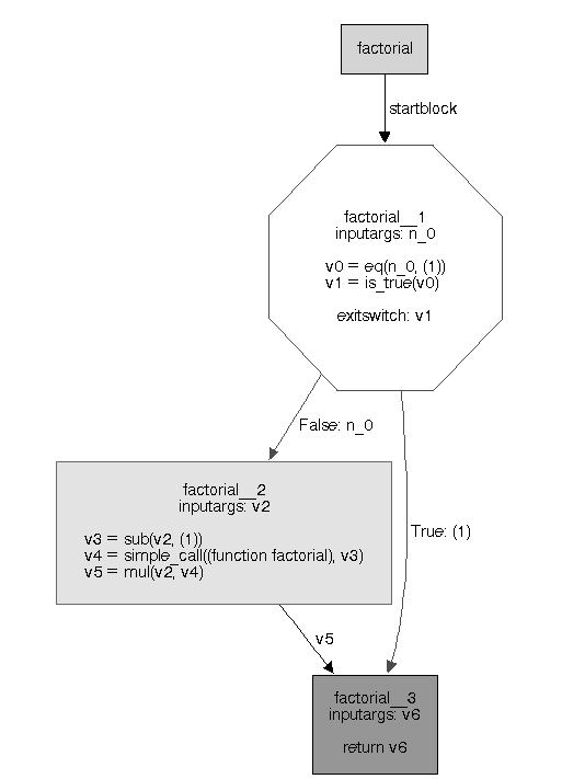
The factorial function has been divided into blocks containing the operations the flowspace recorded. Each block has input arguments and a list of operations on the variables and constants. The first block has an exit switch at the end, which determines which block control-flow will pass to after the first block is run. The exit switch can be based on the value of some variable or whether an exception occurred in the last operation of the block. Control-flow follows the lines between the blocks.
The flow-graph generated in the flow objspace is in static single assignment form, or SSA, an intermediate representation commonly used in compilers. The key feature of SSA is that every variable is only assigned once. This property simplifies the implementation of many compiler transformations and optimizations.
After a function graph is generated, the annotation phase begins. The annotator assigns a type to the results and arguments of each operation. For example, the factorial function above will be annotated to accept and return an integer.
The next phase is called RTyping. RTyping uses type information from the
annotator to expand each high-level flow-graph operation into low-level ones. It
is the first part of translation where the target backend matters. The backend
chooses a type system for the RTyper to specialize the program to. The RTyper
currently has two type systems: A low-level typesystem for backends like C and
one for higher-level typesystems with classes. High-level Python operations and
types are transformed into the level of the type system. For example, an
add operation with operands annotated as integers will generate a
int_add operation with the low-level type system. More complicated
operations like hash table lookups generate function calls.
After RTyping, some optimizations on the low-level flow-graph are performed. They are mostly of the traditional compiler variety like constant folding, store sinking, and dead code removal.
Python code typically has frequent dynamic memory allocations. RPython, being a Python derivative, inherits this allocation intensive pattern. In many cases, though, allocations are temporary and local to a function. Malloc removal is an optimization that addresses these cases. Malloc removal removes these allocations by "flattening" the previously dynamically allocated object into component scalars when possible.
To see how malloc removals works, consider the following function that computes the Euclidean distance between two points on the plane in a roundabout fashion:
def distance(x1, y1, x2, y2):
    p1 = (x1, y1)
    p2 = (x2, y2)
    return math.hypot(p1[0] - p2[0], p1[1] - p2[1])
When initially RTyped, the body of the function has the following operations:
v60 = malloc((GcStruct tuple2))
v61 = setfield(v60, ('item0'), x1_1)
v62 = setfield(v60, ('item1'), y1_1)
v63 = malloc((GcStruct tuple2))
v64 = setfield(v63, ('item0'), x2_1)
v65 = setfield(v63, ('item1'), y2_1)
v66 = getfield(v60, ('item0'))
v67 = getfield(v63, ('item0'))
v68 = int_sub(v66, v67)
v69 = getfield(v60, ('item1'))
v70 = getfield(v63, ('item1'))
v71 = int_sub(v69, v70)
v72 = cast_int_to_float(v68)
v73 = cast_int_to_float(v71)
v74 = direct_call(math_hypot, v72, v73)
This code is suboptimal in several ways. Two tuples that never escape the function are allocated. Additionally, there is unnecessary indirection accessing the tuple fields.
Running malloc removal produces the following concise code:
v53 = int_sub(x1_0, x2_0)
v56 = int_sub(y1_0, y2_0)
v57 = cast_int_to_float(v53)
v58 = cast_int_to_float(v56)
v59 = direct_call(math_hypot, v57, v58)
The tuple allocations have been completely removed and the indirections flattened out. Later, we will see how a technique similar to malloc removal is used on application-level Python in the PyPy JIT (Section 19.5).
PyPy also does function inlining. As in lower-level languages, inlining improves performance in RPython. Somewhat surprisingly, it also reduces the size of the final binary. This is because it allows more constant folding and malloc removal to take place, which reduces overall code size.
The program, now in optimized, low-level flow-graphs, is passed to the backend to generate sources. Before it can generate C code, the C backend must perform some additional transformations. One of these is exception transformation, where exception handling is rewritten to use manual stack unwinding. Another is the insertion of stack depth checks. These raise an exception at runtime if the recursion is too deep. Places where stack depth checks are needed are found by computing cycles in the call graph of the program.
Another one of the transformations performed by the C backend is adding garbage collection (GC). RPython, like Python, is a garbage-collected language, but C is not, so a garbage collector has to be added. To do this, a garbage collection transformer converts the flow-graphs of the program into a garbage-collected program. PyPy's GC transformers provide an excellent demonstration of how translation abstracts away mundane details. In CPython, which uses reference counting, the C code of the interpreter must carefully keep track of references to Python objects it is manipulating. This not only hardcodes the garbage collection scheme in the entire codebase but is prone to subtle human errors. PyPy's GC transformer solves both problems; it allows different garbage collection schemes to be swapped in and out seamlessly. It is trivial to evaluate a garbage collector implementation (of which PyPy has many), simply by tweaking a configuration option at translation. Modulo transformer bugs, the GC transformer also never makes reference mistakes or forgets to inform the GC when an object is no longer in use. The power of the GC abstraction allows GC implementations that would be practically impossible to hardcode in an interpreter. For example, several of PyPy's GC implementations require a write barrier. A write barrier is a check which must be performed every time a GC-managed object is placed in another GC-managed array or structure. The process of inserting write barriers would be laborious and fraught with mistakes if done manually, but is trivial when done automatically by the GC transformer.
The C backend can finally emit C source code. The generated C code, being
generated from low-level flow-graphs, is an ugly mess of gotos and obscurely
named variables. An advantage of writing C is that the C compiler can do most of
the complicated static transformation work required to make a final binary-like
loop optimizations and register allocation.
Python, like most dynamic languages, has traditionally traded efficiency for flexibility. The architecture of PyPy, being especially rich in flexibility and abstraction, makes very fast interpretation difficult. The powerful objspace and multimethod abstractions in the std objspace do not come without a cost. Consequently, the vanilla PyPy interpreter performs up to 4 times slower than CPython. To remedy not only this but Python's reputation as a sluggish language, PyPy has a just-in-time compiler (commonly written JIT). The JIT compiles frequently used codepaths into assembly during the runtime of the program.
The PyPy JIT takes advantage of PyPy's unique translation architecture described in Section 19.4. PyPy actually has no Python-specific JIT; it has a JIT generator. JIT generation is implemented as simply another optional pass during translation. A interpreter desiring JIT generation need only make two special function calls called jit hints.
PyPy's JIT is a tracing JIT. This means it detects "hot" (meaning frequently run) loops to optimize by compiling to assembly. When the JIT has decided it is going to compile a loop, it records operations in one iteration of the loop, a process called tracing. These operations are subsequently compiled to machine code.
As mentioned above, the JIT generator requires only two hints in the interpreter
to generate a JIT: merge_point and
can_enter_jit. can_enter_jit tells the JIT where in the
interpreter a loop starts. In the Python interpreter, this is the end of the
JUMP_ABSOLUTE bytecode. (JUMP_ABSOLUTE makes the interpreter jump
to the head of the app-level loop.) merge_point tells the JIT where it is
safe to return to the interpreter from the JIT. This is the beginning of the
bytecode dispatch loop in the Python interpreter.
The JIT generator is invoked after the RTyping phase of translation. Recall that at this point, the program's flow-graphs consist of low-level operations nearly ready for target code generation. The JIT generator locates the hints mentioned above in the interpreter and replaces them with calls to invoke the JIT during runtime. The JIT generator then writes a serialized representation of the flow-graphs of every function that the interpreter wants jitted. These serialized flow-graphs are called jitcodes. The entire interpreter is now described in terms of low-level RPython operations. The jitcodes are saved in the final binary for use at runtime.
At runtime, the JIT maintains a counter for every loop that is executed in the program. When a loop's counter exceeds a configurable threshold, the JIT is invoked and tracing begins. The key object in tracing is the meta-interpreter. The meta-interpreter executes the jitcodes created in translation. It is thus interpreting the main interpreter, hence the name. As it traces the loop, it creates a list of the operations it is executing and records them in JIT intermediate representation (IR), another operation format. This list is called the trace of the loop. When the meta-interpreter encounters a call to a jitted function (one for which jitcode exists), the meta-interpreter enters it and records its operations to original trace. Thus, the tracing has the effect of flattening out the call stack; the only calls in the trace are to interpreter functions that are outside the knowledge of jit.
The meta-interpreter is forced to specialize the trace to properties of the loop
iteration it is tracing. For example, when the meta-interpreter encounters a
conditional in the jitcode, it naturally must choose one path based on the state
of the program. When it makes a choice based on runtime information, the
meta-interpreter records an IR operation called a guard. In the case of a
conditional, this will be a guard_true or guard_false operation on
the condition variable. Most arithmetic operations also have guards, which
ensure the operation did not overflow. Essentially, guards codify assumptions
the meta-interpreter is making as it traces. When assembly is generated, the
guards will protect assembly from being run in a context it is not specialized
for. Tracing ends when the meta-interpreter reaches the same
can_enter_jit operation with which it started tracing. The loop IR can
now be passed to the optimizer.
The JIT optimizer features a few classical compiler optimizations and many optimizations specialized for dynamic languages. Among the most important of the latter are virtuals and virtualizables.
Virtuals are objects which are known not to escape the trace, meaning they are not passed as arguments to external, non-jitted function calls. Structures and constant length arrays can be virtuals. Virtuals do not have to be allocated, and their data can be stored directly in registers and on the stack. (This is much like the static malloc removal phase described in the section about translation backend optimizations.) The virtuals optimization strips away the indirection and memory allocation inefficiencies in the Python interpreter. For example, by becoming virtual, boxed Python integer objects are unboxed into simple word-sized integers and can be stored directly in machine registers.
A virtualizable acts much like a virtual but may escape the trace (that is, be passed to non-jitted functions). In the Python interpreter the frame object, which holds variable values and the instruction pointer, is marked virtualizable. This allows stack manipulations and other operations on the frame to be optimized out. Although virtuals and virtualizables are similar, they share nothing in implementation. Virtualizables are handled during tracing by the meta-interpreter. This is unlike virtuals, which are handled during trace optimization. The reason for this is virtualizables require special treatment, since they may escape the trace. Specifically, the meta-interpreter has to ensure that non-jitted functions that may use the virtualizable don't actually try to fetch its fields. This is because in jitted code, the fields of virtualizable are stored in the stack and registers, so the actual virtualizable may be out of date with respect to its current values in the jitted code. During JIT generation, code which accesses a virtualizable is rewritten to check if jitted assembly is running. If it is, the JIT is asked to update the fields from data in assembly. Additionally when the external call returns to jitted code, execution bails back to the interpreter.
After optimization, the trace is ready to be assembled. Since the JIT IR is already quite low-level, assembly generation is not too difficult. Most IR operations correspond to only a few x86 assembly operations. The register allocator is a simple linear algorithm. At the moment, the increased time that would be spent in the backend with a more sophisticated register allocation algorithm in exchange for generating slightly better code has not been justified. The trickiest portions of assembly generation are garbage collector integration and guard recovery. The GC has to be made aware of stack roots in the generated JIT code. This is accomplished by special support in the GC for dynamic root maps.
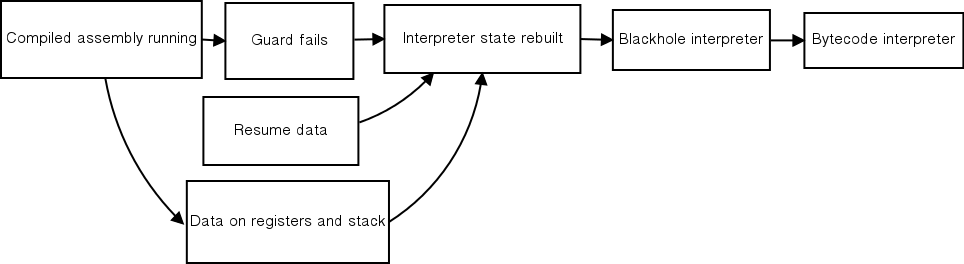
When a guard fails, the compiled assembly is no longer valid and control must return to the bytecode interpreter. This bailing out is one of the most difficult parts of JIT implementation, since the interpreter state has to be reconstructed from the register and stack state at the point the guard failed. For each guard, the assembler writes a compact description of where all the values needed to reconstruct the interpreter state are. At guard failure, execution jumps to a function which decodes this description and passes the recovery values to a higher level be reconstructed. The failing guard may be in the middle of the execution of a complicated opcode, so the interpreter can not just start with the next opcode. To solve this, PyPy uses a blackhole interpreter. The blackhole interpreter executes jitcodes starting from the point of guard failure until the next merge point is reached. There, the real interpreter can resume. The blackhole interpreter is so named because unlike the meta-interpreter, it doesn't record any of the operations it executes. The process of guard failure is depicted in Figure 19.3.
As described up to this point, the JIT would be essentially useless on any loop with a frequently changing condition, because a guard failure would prevent assembly from running very many iterations. Every guard has a failure counter. After the failure count has passed a certain threshold, the JIT starts tracing from the point of guard failure instead of bailing back to the interpreter. This new sub-trace is called a bridge. When the tracing reaches the end of the loop, the bridge is optimized and compiled and the original loop is patched at the guard to jump to the new bridge instead of the failure code. This way, loops with dynamic conditions can be jitted.
How successful have the techniques used in the PyPy JIT proven? At the time of this writing, PyPy is a geometric average of five times faster than CPython on a comprehensive suite of benchmarks. With the JIT, app-level Python has the possibility of being faster than interp-level code. PyPy developers have recently had the excellent problem of having to write interp-level loops in app-level Python for performance.
Most importantly, the fact that the JIT is not specific to Python means it can be applied to any interpreter written within the PyPy framework. This need not necessarily be a language interpreter. For example, the JIT is used for Python's regular expression engine. NumPy is a powerful array module for Python used in numerical computing and scientific research. PyPy has an experimental reimplementation of NumPy. It harnesses the power of the PyPy JIT to speed up operations on arrays. While the NumPy implementation is still in its early stages, initial performance results look promising.
While it beats C any day, writing in RPython can be a frustrating experience. Its implicit typing is difficult to get used to at first. Not all Python language features are supported and others are arbitrarily restricted. RPython is not specified formally anywhere and what the translator accepts can vary from day to day as RPython is adapted to PyPy's needs. The author of this chapter often manages to create programs that churn in the translator for half an hour, only to fail with an obscure error.
The fact that the RPython translator is a whole-program analyzer creates some practical problems. The smallest change anywhere in translated code requires retranslating the entire interpreter. That currently takes about 40 minutes on a fast, modern system. The delay is especially annoying for testing how changes affect the JIT, since measuring performance requires a translated interpreter. The requirement that the whole program be present at translation means modules containing RPython cannot be built and loaded separately from the core interpreter.
The levels of abstraction in PyPy are not always as clear cut as in theory. While technically the JIT generator should be able to produce an excellent JIT for a language given only the two hints mentioned above, the reality is that it behaves better on some code than others. The Python interpreter has seen a lot of work towards making it more "jit-friendly", including many more JIT hints and even new data structures optimized for the JIT.
The many layers of PyPy can make tracking down bugs a laborious process. A Python interpreter bug could be directly in the interpreter source or buried somewhere in the semantics of RPython and the translation toolchain. Especially when a bug cannot be reproduced on the untranslated interpreter, debugging is difficult. It typically involves running GDB on the nearly unreadable generated C sources.
Translating even a restricted subset of Python to a much lower-level language like C is not an easy task. The lowering passes described in Section 19.4 are not really independent. Functions are being annotated and rtyped throughout translation, and the annotator has some knowledge of low-level types. The RPython translator is thus a tangled web of cross-dependencies. The translator could do with cleaning up in several places, but doing it is neither easy nor much fun.
In part to combat its own complexity (see Section 19.6), PyPy has adopted several so-called "agile" development methodologies. By far the most important of these is test-driven development. All new features and bug fixes are required to have tests to verify their correctness. The PyPy Python interpreter is also run against CPython's regression test suite. PyPy's test driver, py.test, was spun off and is now used in many other projects. PyPy also has a continuous integration system that runs the test suite and translates the interpreter on a variety of platforms. Binaries for all platforms are produced daily and the benchmark suite is run. All these tests ensure that the various components are behaving, no matter what change is made in the complicated architecture.
There is a strong culture of experimentation in the PyPy project. Developers are encouraged to make branches in the Mercurial repository. There, ideas in development can be refined without destabilizing the main branch. Branches are not always successful, and some are abandoned. If anything though, PyPy developers are tenacious. Most famously, the current PyPy JIT is the fifth attempt to add a JIT to PyPy!
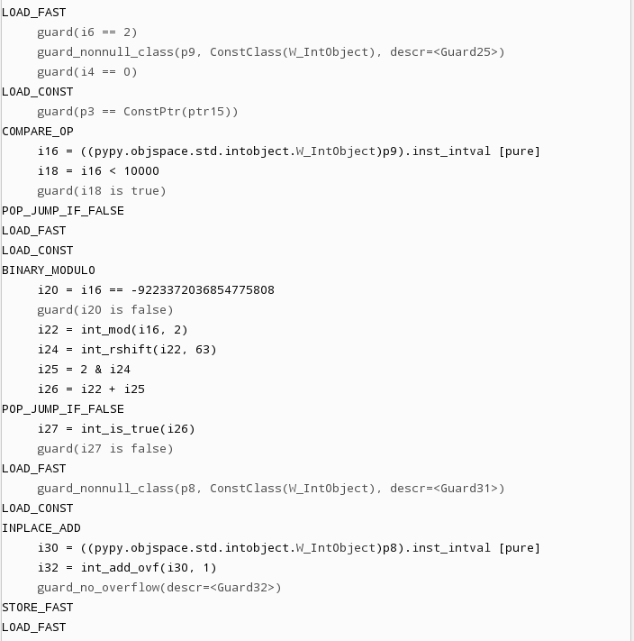
The PyPy project also prides itself on its visualization tools. The flow-graph charts in Section 19.4 are one example. PyPy also has tools to show invocation of the garbage collector over time and view the parse trees of regular expressions. Of special interest is jitviewer, a program that allows one to visually peel back the layers of a jitted function, from Python bytecode to JIT IR to assembly. (The jitviewer is shown in Figure 19.4.) Visualization tools help developers understand how PyPy's many layers interact with each other.
The Python interpreter treats Python objects as black boxes and leaves all behavior to be defined by the objspace. Individual objspaces can provide special extended behavior to Python objects. The objspace approach also enables the abstract interpretation technique used in translation.
The RPython translator allows details like garbage collection and exception handling to be abstracted from the language interpreter. It also opens up the possibly of running PyPy on many different runtime platforms by using different backends.
One of the most important uses of the translation architecture is the JIT generator. The generality of the JIT generator allows JITs for new languages and sub-languages like regular expressions to be added. PyPy is the fastest Python implementation today because of its JIT generator.
While most of PyPy's development effort has gone into the Python interpreter, PyPy can be used for the implementation of any dynamic language. Over the years, partial interpreters for JavaScript, Prolog, Scheme, and IO have been written with PyPy.
Finally, some of lessons to take away from the PyPy project:
Repeated refactoring is often a necessary process. For example, it was originally envisioned that the C backend for the translator would be able to work off the high-level flow graphs! It took several iterations for the current multi-phase translation process to be born.
The most important lesson of PyPy is the power of abstraction. In PyPy, abstractions separate implementation concerns. For example, RPython's automatic garbage collection allows a developer working the interpreter to not worry about memory management. At the same time, abstractions have a mental cost. Working on the translation chain involves juggling the various phases of translation at once in one's head. What layer a bug resides in can also be clouded by abstractions; abstraction leakage, where swapping low-level components that should be interchangeable breaks higher-level code, is perennial problem. It is important that tests are used to verify that all parts of the system are working, so a change in one system does not break a different one. More concretely, abstractions can slow a program down by creating too much indirection.
The flexibility of (R)Python as an implementation language makes experimenting with new Python language features (or even new languages) easy. Because of its unique architecture, PyPy will play a large role in the future of Python and dynamic language implementation.